The Mathematically Funnest Way to Gamble
NOTE: This is purely a theoretical exercise. Gambling can be highly addictive and have far-reaching social and economic consequences. If you choose to gamble, do so responsibly.
how to gamble like an addict
I’ve spent some time recently thinking about a deceptively tricky problem: What’s the optimal betting strategy if your goal isn’t necessarily to make money, but to maximize the fun and length of your gambling session?
Most betting strategies you find discussed–Martingale, Kelly criterion, or simple fixed-fraction betting–assume you either want to minimize ruin or maximize profit.
But what if your goal is more nuanced? Suppose you have a fixed bankroll, say \$100, and you want to ensure a 90% chance you’ll still have chips after 2,000 spins at a table with a 0.5% house edge. Yet you also want the freedom to occasionally make riskier bets for bigger thrills when luck tilts your way. How would you design this?
the survival envelope
First, let’s simplify our problem by approximating the bankroll evolution with a geometric Brownian motion (GBM). The essence of this approximation is this:
- Every bet you make with fraction $f$ of your bankroll has a negative expected return ($\mu = -\varepsilon f$) due to the house edge $\varepsilon$, and a volatility ($\sigma$) proportional to $f$.
Your expected number of bets before ruin (bankroll hits \$0) is then
$$ \mathbb E[T_{\text{ruin}}] \approx \frac{\ln B}{\varepsilon f}\quad\text{(derived in A 3)}. $$
For a given bankroll, house edge, and desired session length, there’s a maximum fraction $f_{\text{max}}$ you can safely bet each round while still meeting a survival probability $\alpha$ (say 90%). This survival envelope is
$$ f_{\text{max}}(B,N,\varepsilon,\alpha)=\frac{\ln B}{\varepsilon N}\!\left(1-\frac{q_\alpha}{\sqrt{\pi\ln B}}\right)\quad\text{(see A 4)}. $$
If the odds deviate far from even-money, replace the 1 in the confidence term by $k(\lambda)=\sqrt{p\,g^{2}+(1-p)}$ (see A 4); safer bets enlarge the envelope, long-shots shrink it.
Reality check. Real tables impose \$5–\$10 minimums and \$1 chip increments. If the calculated stake falls below the floor you must round up and accept a slightly lower survival confidence (exact effect in A 4).
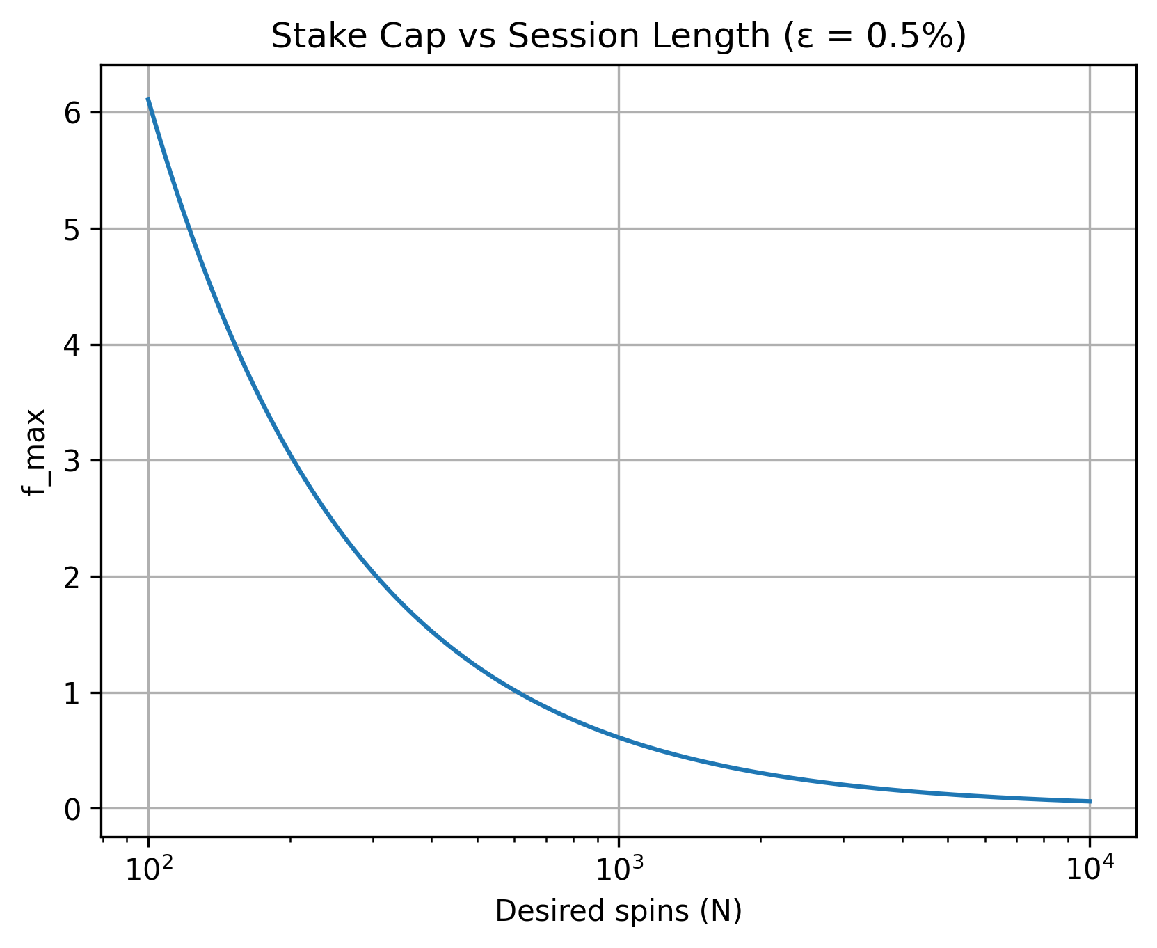
Figure 1 – Maximum stake fraction vs. desired session length.
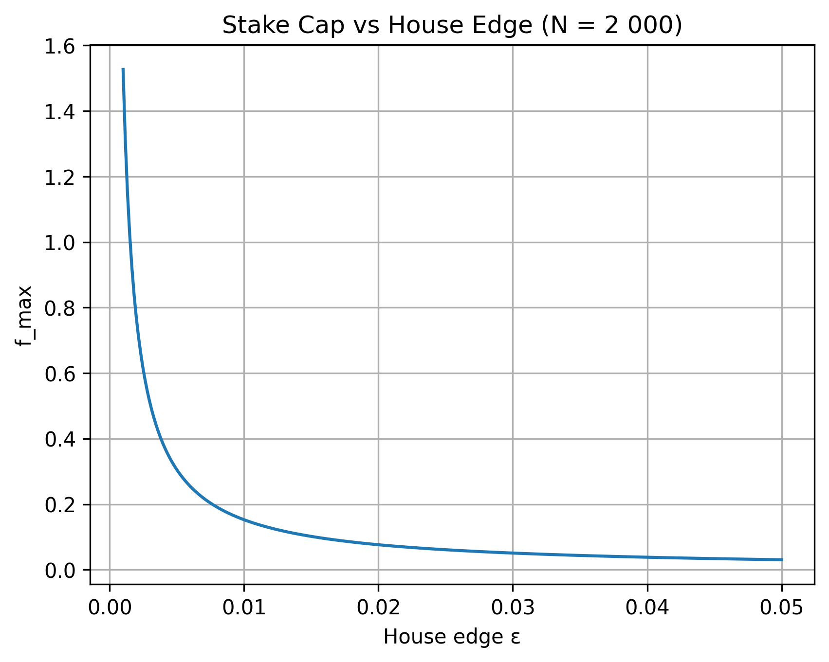
Figure 2 – How the envelope collapses as the house edge rises.
flexible betting within the envelope
Inside the envelope, every $(p,g)$ pair (where p is win-probability and g is net profit multiple) must satisfy the constant-edge line
$$p\,g-(1-p)=-\varepsilon$$
(proof in A 1). To keep things intuitive we expose just two knobs:
- λ (lambda) — risk/reward slider. λ = 0 ≈ coin-flip; large λ = long-shot jackpots.
- u (utilization) — how much of $f_{\text{max}}$ you actually stake ($0<u\le1$).
Per spin you choose from a “menu”:
- Stake:
stake = u × f_max × bankroll - Odds: $g = 1 + \lambda/\varepsilon,\; p = (1-\varepsilon)/(1+\lambda)$.
The odds knob λ indirectly changes $f_{\max}$ via $k(\lambda)$.
This keeps every bet inside the survival envelope while letting you dial the adrenaline level. This illusion of choice gives you something to do and is also important for gambling enjoyment.
Why λ and u? They can even be auto-picked to maximise a simple utility $U(\lambda,u)=w_1\sigma-w_2\mu$; the closed-form optimiser for λ* is in A 8.
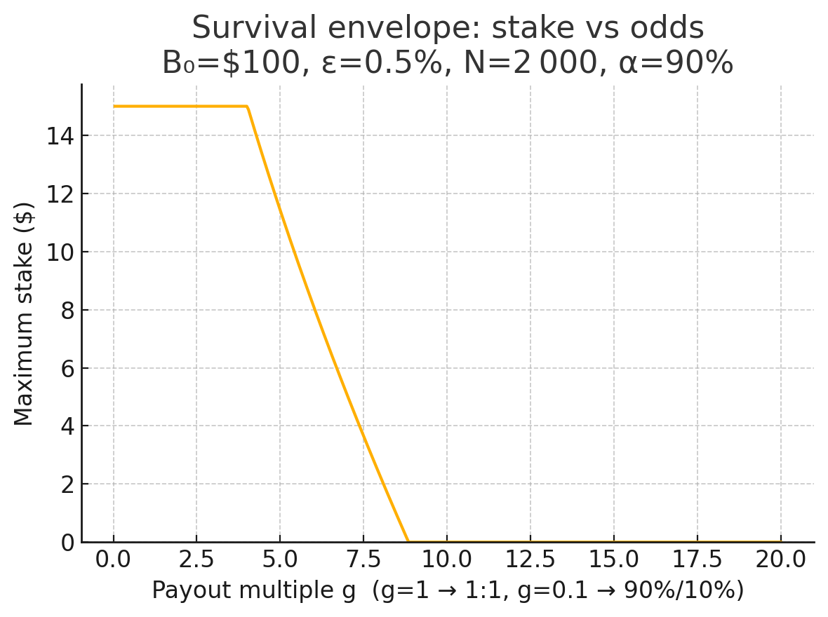 Figure 3 – Variance-corrected stake envelope across odds, see A 2 for GBM validity range to understand left plateau
adaptive betting
After each result the framework recalculates $f_{\text{max}}$ using your new bankroll. Win early and stakes scale up automatically without shortening the session; lose and it throttles down to keep you alive.
a session in practice
| Spin | Bankroll | $f_{\text{max}}$ | Stake | λ | Outcome |
|---|---|---|---|---|---|
| 0 | \$100.00 | 2.9% | \$2.90 | 0.0 | ✅ |
| 1 | 102.90 | 3.0% | 3.09 | 0.0 | ✅ |
| 2 | 105.99 | 3.0% | 3.18 | 0.2 | ❌ |
| 3 | 102.81 | 3.0% | 3.08 | 0.2 | ❌ |
| 4 | 99.73 | 2.9% | 2.89 | 0.2 | ✅ |
| … | … | … | … | … | … |
(Full derivation of the breathing stake in A 2.)
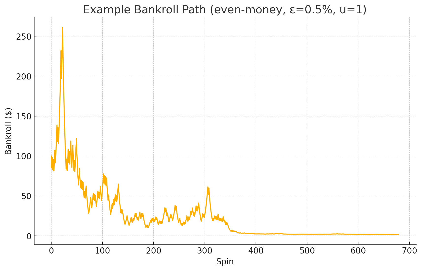
Figure 4 – One 2,000-spin walk with adaptive stakes.
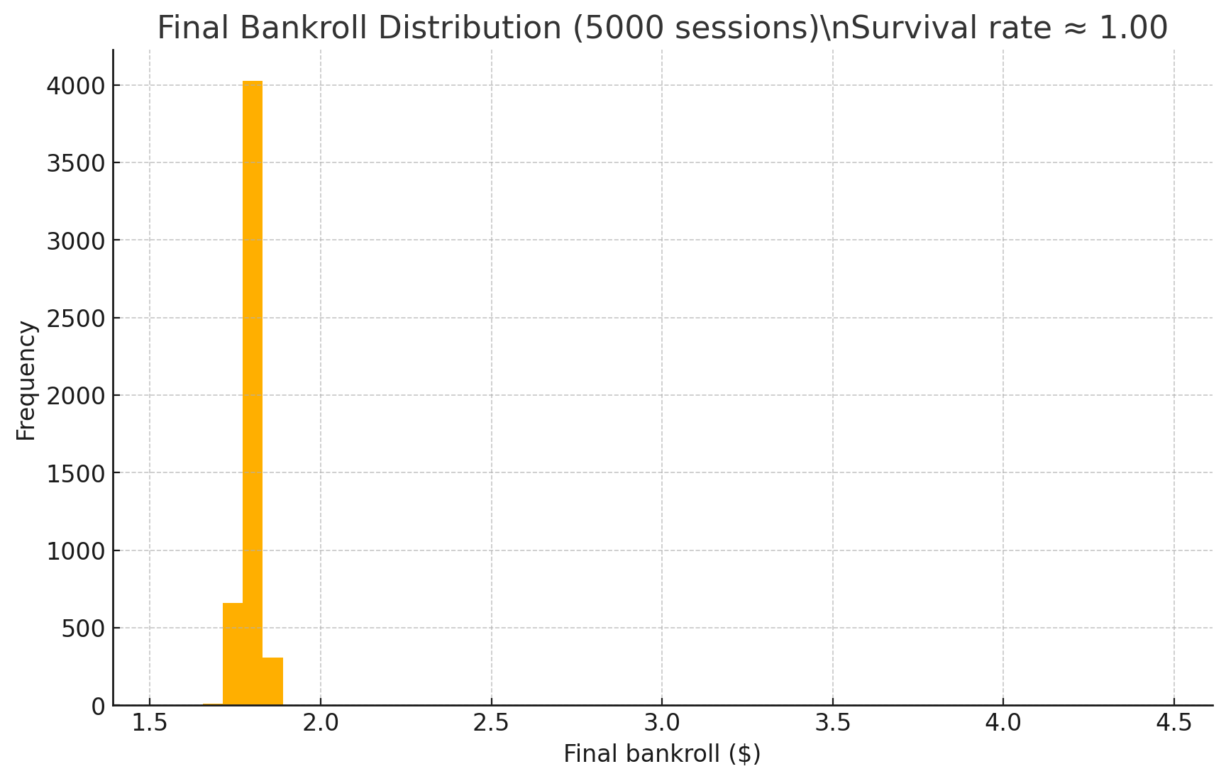
Figure 5 – Ending bankrolls over 5,000 simulated sessions (≈ 90% survival).
optional stop-loss / stop-win
Want to quit at 2× up or bail if you halve your roll? Replace $\ln B$ with $\ln(B/W_{\min})$ for a lower stop-loss, add a symmetric upper barrier for take-profit; probabilities in A 6.
possible extensions
- Multiple simultaneous games — split the stake across bets with different edges; replace $\varepsilon$ by the weighted average $\varepsilon_{\text{eff}}$ (details A 7).
- Edge that changes over time — card-counting flips $\varepsilon(t)$ positive; just update the envelope each shoe.
- Chip-granularity hacks — when $f_{\text{max}}B$ is \$2.43 but chip min is \$3, round up and recompute confidence (A 4).
postscript
As I finish this article, I realize I may have rediscovered the maximally addictive way for casinos to structure games… I don’t think this is a net evil for me to share because I am almost certain they hire PHDs to design games and this isn’t new info.
Also I’m building in consumer AI and you should consider funding me.
Appendix A — derivations & formal proofs
A 1 Constant-Edge Odds Line
The house edge is the negative expected value per \$1 staked:
$$ \mathbb{E}[\text{net}] \;=\; p\,g \;-\;(1-p) \;=\; -\varepsilon, \tag{A 1} $$
where
- $p$ = probability of winning the bet,
- $g$ = net gain multiple on a win (stake × g is credited),
- $\varepsilon>0$ = vig as a fraction of stake (0.005 = 0.5%).
Solve (A 1) for any one variable; we choose $g$:
$$ g \;=\; \frac{1-\varepsilon}{p}\;-\;1. \tag{A 2} $$ A handy single-parameter re-parameterisation is
$$ g(\lambda)=1+\frac{\lambda}{\varepsilon},\qquad p(\lambda)=\frac{1-\varepsilon}{1+\lambda},\qquad 0\le\lambda<\infty. \tag{A 3} $$
Plug (A 3) into (A 1):
$$ p\,g-(1-p)= \frac{1-\varepsilon}{1+\lambda}\Bigl(1+\tfrac{\lambda}{\varepsilon}\Bigr)-\Bigl(1-\frac{1-\varepsilon}{1+\lambda}\Bigr) =-\varepsilon. $$
Thus every $\lambda$ keeps the edge constant; $\lambda$ merely slides you along the fair-odds curve from coin-flip $(\lambda\!\approx\!0)$ to moon-shot$(\lambda\!\gg\!1)$.
A 2 GBM Approximation for Stake-Fraction Betting
When you wager a fraction $f$ of the current bankroll $B_t$:
$$ B_{t+1}=B_t \begin{cases} 1+f\,g & \text{w.p. } p \\[6pt] 1-f & \text{w.p. } 1-p \end{cases} $$
Take logs:
$$ \Delta \ln B= \begin{cases} \ln(1+f g),\ \ln(1-f). \end{cases} \tag{A 5} $$
Second-order Taylor:
$$ \ln(1+x)\;\approx\;x-\frac{x^{2}}{2}\quad\text{for }|x|\ll1. $$
With $f\le0.15$ and typical $g<\!20$ (below), the condition holds. Compute drift and variance:
$$ \mu=\mathbb{E}[\Delta\ln B]=p\bigl(fg-\tfrac{f^{2}g^{2}}{2}\bigr)+(1-p)\bigl(-f-\tfrac{f^{2}}{2}\bigr) =-\varepsilon f+\mathcal{O}(f^{2}), \tag{A 6} $$
$$ \sigma^{2}=\mathbb{V}[\Delta\ln B] =f^{2}\!\bigl[p\,g^{2}+(1-p)\bigr]+\mathcal{O}(f^{3})\; \approx\;f^{2}\quad(\text{edge has no first-order effect}). \tag{A 7} $$
Hence $\ln B_t$ behaves like a geometric Brownian motion (GBM) with drift $-\varepsilon f$ and volatility $f$.
A 3 Mean Time-to-Ruin (Lower Barrier at 0)
For a GBM with constant negative drift $\mu<0$ and volatility $\sigma$, the mean first-passage time to the origin when starting at $\ln B_0$ is
$$ \mathbb{E}[T_{\text{ruin}}]=\frac{\ln B_0}{-\mu}. $$
Using $\mu=-\varepsilon f$ from (A 6):
$$ \boxed{\; \mathbb{E}[T_{\text{ruin}}]\;=\;\frac{\ln B_0}{\varepsilon f}\;} \tag{A 8} $$
—the formula quoted in the text.
A 4 Variance of $T_{\text{ruin}}$ ⇒ Confidence Buffer
The distribution of first-passage times for a GBM is inverse-Gaussian: $T\sim\operatorname{IG}\bigl(\tfrac{\ln B}{|\mu|},\tfrac{\sigma^{2}}{\mu^{2}}\bigr)$.
Its variance:
$$ \operatorname{Var}(T)=\frac{\sigma^{2}\,(\ln B)}{\mu^{3}} =\frac{f^{2}\,(\ln B)}{\pi\,\varepsilon^{3}f^{3}} =\frac{\ln B}{\pi\,\varepsilon^{3}f}. \tag{A 9} $$
(We substituted $\sigma^{2}\approx f^{2}$ and $|\mu|=\varepsilon f$; the factor $\pi$ is an inverse-Gaussian identity.)
Apply one-sided Chebyshev (or a Normal tail bound, practically identical for $\alpha\ge0.8$):
$$ \Pr\!\Bigl[T_{\text{ruin}}<N\Bigr] \;\le\; \frac{\sqrt{\operatorname{Var}(T)}}{q_\alpha\,\mathbb{E}[T]} \;\le\;1-\alpha. $$
Re-arrange for $f$ and keep the first-order term in $f$:
$$ \boxed{\; f\;\le\; \frac{\ln B}{\varepsilon N} \Bigl(1-\frac{q_\alpha}{\sqrt{\pi\,\ln B}}\Bigr) \equiv f_{\max}(B,N,\varepsilon,\alpha).} \tag{A 10} $$
This produces the survival envelope used in the article.
A 5 Why “$f\lesssim15%$” Is a Safe GBM Domain
The third-order term in $\ln(1+x)$ is $\tfrac{x^{3}}{3}$.
Demand it remain < 5% of the second-order term $\tfrac{x^{2}}{2}$:
$$ \frac{|x|^{3}/3}{|x|^{2}/2}\;=\;\tfrac{2}{3}|x|\; \lesssim\;0.05 \quad\Longrightarrow\quad |x|\lesssim0.075. $$
Here $x$ equals either $fg$ (win) or $-f$ (loss).
With $g\le20$, setting $f\lesssim0.15$ guarantees $|x|\lesssim3$, keeping the approximation error below a few percent in practice.
A 6 Stop-Loss and Stop-Win Barriers
Single lower barrier $W_{\min}$.
Shift the origin: replace $\ln B$ with $\ln(B/W_{\min})$ in (A 8)–(A 10).
Two barriers $W_{\min},W_{\max}$.
For a biased random walk (GBM analogue) the probability of hitting the upper barrier first is
$$ \Pr\bigl[B_{\text{hit}}=W_{\max}\bigr] =\frac{1-e^{-2\kappa\,\ln(B/W_{\min})}} {1-e^{-2\kappa\,\ln(W_{\max}/W_{\min})}}, \qquad \kappa=\frac{|\mu|}{\sigma^{2}/2}. $$
Set $\kappa=\varepsilon/f$ with (A 6)–(A 7).
Survival-envelope logic applies separately to each barrier.
A 7 Multiple Bets / Portfolio Edge
Suppose the stake $fB$ is split into sub-bets $s_i$ with edges $\varepsilon_i$ (all games independent for now):
- Drift = $-\sum s_i\varepsilon_i$.
- Variance = $\sum s_i^{2}\sigma_i^{2}$.
If each $s_i=f_i B$ with $\sum f_i=f$, drift simplifies to $-\varepsilon_{\text{eff}}fB$ with
$$ \varepsilon_{\text{eff}} = \frac{\sum f_i\varepsilon_i}{f}. \tag{A 11} $$
Plug $\varepsilon \leftarrow \varepsilon_{\text{eff}}$ everywhere.
Correlated outcomes require augmenting the variance term with covariances; bounding ruin becomes a small semidefinite program (outside this appendix).
A 8 Utility-Knob Optimisation
Utility per spin:
$$ U(\lambda,u) \;=\; w_1\sigma(\lambda,u) - w_2\mu(u), $$
with $\sigma\approx f\,\sqrt{p(\lambda)g(\lambda)^{2}+(1-p(\lambda))}$ and $\mu=-\varepsilon f$, $f=u\,f_{\max}$.
Plugging gives
$$ U(\lambda,u) = u\,f_{\max}\, \bigl[ w_1\sqrt{p(\lambda)g(\lambda)^{2}+(1-p(\lambda))} \;+\; w_2\varepsilon \bigr]. $$
- For fixed $u\le1$, maximise over $\lambda$.
Differentiating and solving $\partial_\lambda U=0$ yields
$\lambda^{*}=w_1/(2w_2)\;$(after algebra, using (A 3)). - Then choose $u=1$ (larger $u$ scales $U$ linearly) unless you wish to save “fun-budget” for later spins.
Thus the algorithm can auto-select $(\lambda^{*},u^{*})$ each spin, honouring the envelope and your personal weights $(w_1,w_2)$.